# required packages
library(tidyverse)
library(DT)
library(cleanR)

# load raw data
moda_data <- cleanR::survey_data %>% # converting HDDS variables to numeric
mutate(across(starts_with("HDDS"), as.numeric))Cleaning Food Security Indicators
R programming
Data Cleaning
This guide shows how to clean food security and livelihood data using the cleanR package. we will go through step-by-step from raw data to clean dataset by applying standard checks, reviewing flagged records and preparing clean data ready for analysis. WFP SurveyDesigner 1 codebook is adopted for variable naming and format.
The data cleaning process follows four steps of running checks, reviewing flagged records, apply corrections and export clean dataset at the end.
Step 1: Load data
The first step is to prepare the data by downloading the raw version from the server 2. remember that the documentation is using WFP codebook therefore consider to adopt the codebook if you’re at the planning stage of your assessment. otherwise if you already have data and want to follow the guide try to reshape your data to match the codebook variable naming.
Now that we have the dataset ready, the next step is to calculate indicators.
Step 2: Format data
Now we have prepared the raw data, so we’ll use the calculate_fsl_indicators function to compute the food security and livelihood outcome indicators 3. the function will take arguments of raw data, food consumption score (FSC), reduced coping strategies (rCSI), household hunger scale (HHS), household dietary diversity (HDDS) and the livelhood coping strategeis (LCS-FS) variables.
raw_data <- calculate_fsl_indicators(data = moda_data,
                                 # FCS
                                 FCSStap = "FCSStap",
                                 FCSPulse = "FCSPulse",
                                 FCSPr = "FCSPr",
                                 FCSVeg = "FCSVeg",
                                 FCSFruit = "FCSFruit",
                                 FCSDairy = "FCSDairy",
                                 FCSFat = "FCSFat",
                                 FCSSugar = "FCSSugar",
                                 cutoff = "Cat28",
                                 # rCSI
                                 rCSILessQlty = "rCSILessQlty",
                                 rCSIBorrow = "rCSIBorrow",
                                 rCSIMealSize = "rCSIMealSize",
                                 rCSIMealAdult = "rCSIMealAdult",
                                 rCSIMealNb = "rCSIMealNb",
                                 # HHS
                                 HHhSNoFood_FR = "HHhSNoFood_FR",
                                 HHhSBedHung_FR = "HHhSBedHung_FR",
                                 HHhSNotEat_FR = "HHhSNotEat_FR",
                                 # HDDS
                                 HDDSStapCer = "HDDSStapCer",
                                 HDDSStapRoot = "HDDSStapRoot",
                                 HDDSVeg = "HDDSVegGre",
                                 HDDSFruit = "HDDSFruitOrg",
                                 HDDSPrMeat = "HDDSPrMeatF",
                                 HDDSPrEgg = "HDDSPrEgg",
                                 HDDSPrFish = "HDDSPrFish",
                                 HDDSPulse = "HDDSPulse",
                                 HDDSDairy = "HDDSDairy",
                                 HDDSFat = "HDDSFat",
                                 HDDSSugar = "HDDSSugar",
                                 HDDSCond = "HDDSCond"
                                 )
NotePlease Note
you’ll only need to provide the variable names of the indicators you want to include in your checks and its not required to specify all variables at all times (for instance, if you have data for FCS and rCSI only provide the arguments of these two indicators only).
Step 3: Data Checks
In this step we run the fsl_cleaning_log function to flag all records that may need review.
fsl_clog <- fsl_cleaning_log(data = raw_data, uuid = "uuid")

DT::datatable(head(fsl_clog, 5), options = list(dom = 't'))
After runing the checks, the dataset will include flags that highlight records needing review. these flags do not mean the data is wrong but rather they show where we should closer look.
Basic Checks
These checks help us identify general issues with the dataset. survey duration, other responses and missing/incomplete values are part of the general basic data checks.
Food Consumption Checks
These checks will focus on how often the different food groups are consumed.
- very low cereal or oil consumption (<= 3 days)
- very high meat and dairy consumption (>= 6 days)
- unusual patterns across food groups
For example, cereals are usually consumed frequently. if cereals are very low while other foods are high this may need to be checked.
Consistency checks
These checks compare related indicators to see if they are aligning.
- high meat/dairy consumption with low cereals
- high food consumption with high coping strategies
- mismatch between food consumption and other reduced coping strategies
This situation may indicate inconsistent responses.
Pattern checks
These checks help identify repeated or unusual response patterns.
- same values repeated (7,7,7,7,7)
- altering values (2,1,2,1,2,1,2)
These patterns may suggest rushed or non-careful data entry which is data falsification.
Assuming at this stage that you already run the standard high frequency checks on the data like survey time taken, sample and quota verification and overall survey and operator productivity checks. in this section we’ll go beyond the general checks and perform in-dept data checks.
Lets first use the fsl_cleaning_log function to flag major inconsistency and anomalies in the data. the function will take data and uuid as input and then return cleaning log file with all issues found in the data. this function is now considering critical indicators validation measures.
key checks included in the fsl_cleaning_log function will go as below
| Check | Description |
|---|---|
| Low staple consumption | Flags households reporting very low consumption of staple foods such as cereals or oil, for example cereals or oil consumed for 2 days or less. Since staple foods are usually consumed frequently, very low values may indicate unusual responses or recording errors. |
| All FCS food groups are reported as 7 days | Flags households where all food groups are reported as consumed every day. This may indicate straight-line responses or poor-quality data entry and should be verified. |
| Extreme food group consumption | Reviews food groups with unusually low or high reported consumption frequencies, such as 0–1 days or 6–7 days. This helps identify irregular reporting patterns that may influence the Food Consumption Score. |
| Low cereal or staple consumption while other food groups are reported high | Flags households reporting low cereal or staple consumption while other food groups are consumed frequently. This is an unusual pattern and should be reviewed, especially where cereals or staples are normally the main food source. |
| High meat or dairy consumption with low staples | Flags households reporting frequent consumption of meat or dairy while staple consumption is low, for example meat or dairy consumed 6 days or more while cereals are consumed 4 days or less. This pattern may suggest inconsistency in the food consumption module. |
| High animal-source foods with high coping | Flags households reporting frequent meat or dairy consumption while also reporting high rCSI. This may be inconsistent since high animal-source food consumption usually reflects better food access, while high rCSI reflects stress in accessing food. |
| Acceptable FCS with high rCSI or severe hunger | Flags households with acceptable food consumption but high coping or severe hunger. This may show a contradiction between consumption, coping, and hunger indicators and should be reviewed. |
| High rCSI with very high FCS | Flags households reporting very high food consumption together with high rCSI. This pattern needs validation because high consumption and high coping may not always align. |
| Poor or borderline FCS with all rCSI coping strategies reported as zero | Flags households with poor or borderline food consumption but no reported coping strategies. This may indicate under-reporting of coping strategies or weak probing during the interview. |
| All rCSI coping strategies are reported as 7 days | Flags households where all reduced coping strategies are reported as used every day. This may indicate straight-line responses or poor-quality data entry and should be verified. |
| Adult meal reduction is high, but no reduction in meal size or number of meals is reported | Flags households reporting high adult meal reduction while reporting no reduction in meal size or number of meals. This may indicate inconsistency within the coping strategy responses. |
| Severe hunger scale with acceptable FCS and low rCSI | Flags households reporting severe hunger while also reporting acceptable FCS and low rCSI. This is a possible contradiction between hunger, consumption, and coping indicators and should be reviewed. |
| Repeated response patterns across food groups or coping strategies | Detects repeated or structured response patterns, such as all values reported as 7, or alternating values such as 2,1,2,1. These patterns may indicate enumerator shortcuts, weak probing, or incorrect data entry. |
| Same response pattern repeated across many households by one enumerator | Flags cases where many households interviewed by the same enumerator have identical or very similar food consumption or coping patterns. This may indicate enumerator bias, repeated entry, or field-level data quality issues. |
Step 4: Using Visualizations
By incorporating ridge charts into your analysis, you can easily identify patterns and variations in FCS and rCSI across different clusters or operators.
(plot_ridge_distribution(raw_data, numeric_cols = c("FCSStap", "FCSPulse", "FCSPr", "FCSVeg", "FCSFruit", "FCSDairy", "FCSFat", "FCSSugar"),
                         name_groups = "Food Groups", name_units = "Days", grouping = "EnumName"))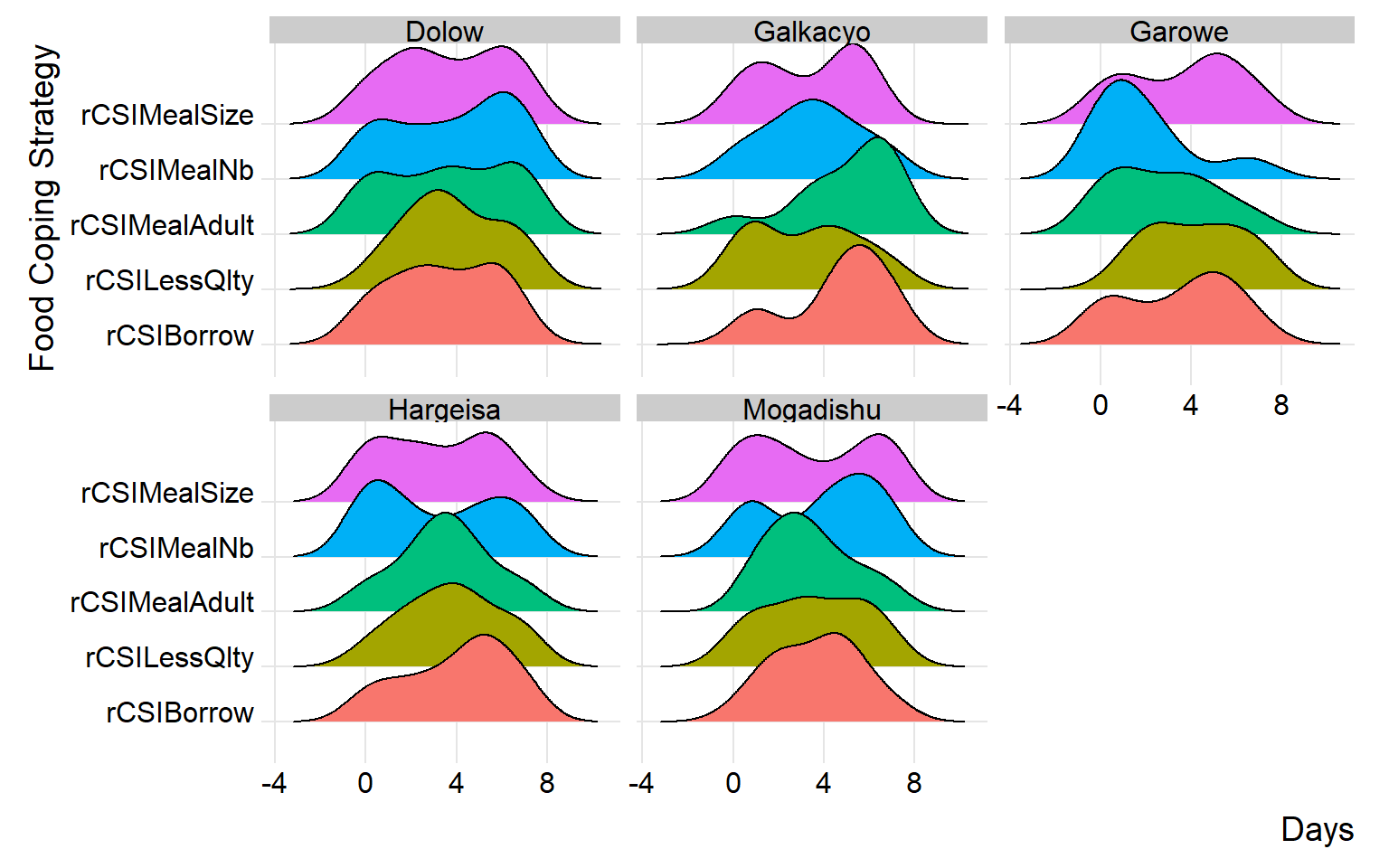
above chart will show the frequency distribution of food groups reported by operator. this visual will help us to identify any anomalies made by the operators. e.g if one operator reports major zero consumption of oil/cereal or sweets it could make alert that there is something need to check from that operators records and debrief them.
(plot_ridge_distribution(raw_data, numeric_cols = c("rCSILessQlty", "rCSIBorrow", "rCSIMealSize", "rCSIMealAdult", "rCSIMealNb"),
                         name_groups = "Food Coping Strategy", name_units = "Days", grouping = "EnumName"))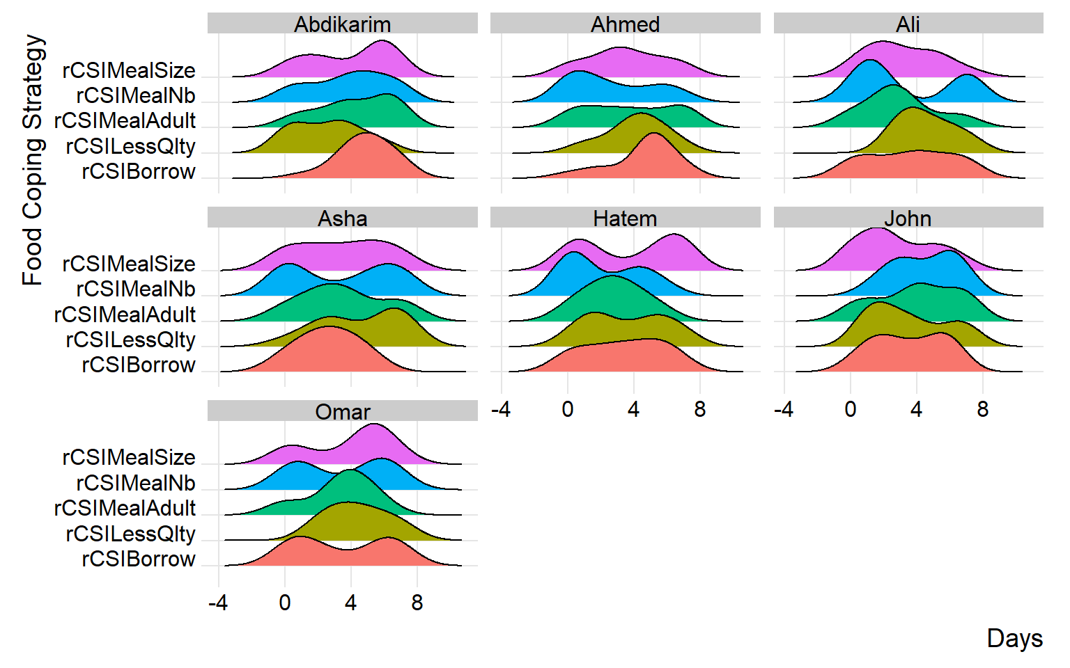
Frequency of reduced coping strategies reported by operator can be found below. similarly this visual will help us to detect if there is inconsistency or anomalies at the operator level.
Step 5: Statistical Checks
As food consumption improves, households tend to use fewer negative coping strategies. This means there is a negative correlation between food consumption and coping strategies. The analysis below shows this correlation overall, and also breaks it down by operator.
Since both food consumption and coping strategies are measured over the same recall period, households that eat a variety of food groups are less likely to skip meals, reduce portion sizes, or borrow food. Based on this relationship, we use the correlation coefficient to identify operators where this trend is weaker or stronger.
correlation <- cor(raw_data$FCS, raw_data$rCSI, use = "complete.obs", method = "pearson")


ggplot(raw_data, aes(x = FCS, y = rCSI)) +
  geom_point(alpha = 0.6, color = "steelblue") +
  geom_smooth(method = "lm", se = TRUE, color = "darkred") +
  labs(
    title = "Relationship between Food Consumption Score and rCSI",
    x = "Food Consumption Score (FCS)",
    y = "Reduced Coping Strategy Index (rCSI)"
  ) +
  theme_minimal() + facet_wrap(~ EnumName)
#> `geom_smooth()` using formula = 'y ~ x'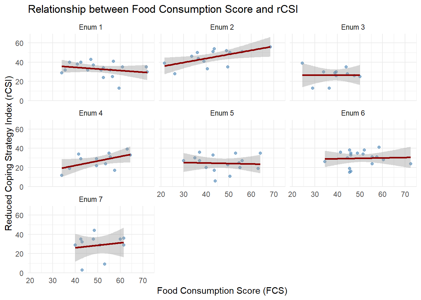
NotePlease Note
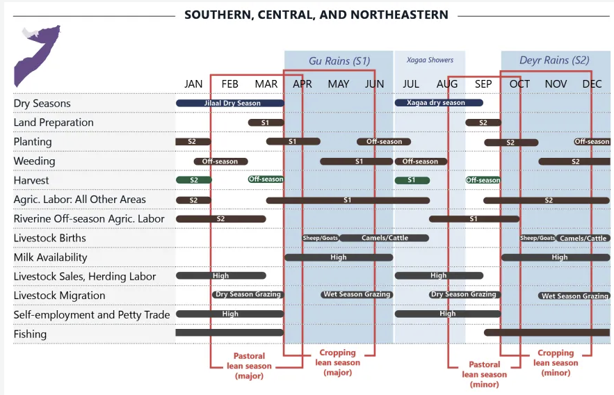
Now that we have explored the data patterns and have some questions, lets see how the data alings with the seasonal calender. for instance Milk availability is hight during the rainy seasons (in the context of Somalia - April - June and October - December). so during these period we should also anticipate higher consumption of dairy and dairy products. so we need to see how our data is aligning with the seasonal calendar and try to understand deeper for any variances spotted.